import numpy as np
import pandas as pd
import IPython.display as ipd
from sklearn.preprocessing import normalize
from matplotlib import pyplot as plt
from scipy.linalg import circulant

from utils.chord_tools import compute_chromagram_from_filename, chord_recognition_template, get_chord_labels, convert_chord_ann_matrix
from utils.chord_tools import compute_eval_measures, plot_matrix_chord_eval
from utils.plot_tools import *6.3. HMM 기반 화음 인식
HMM-Based Chord Recognition
화음인식
HMM
Viterbi
HMM(Hidden Markov Model)과 Viterbi 알고리즘을 설명하고 HMM 기반 화음 인식 방법과 그 예를 다룬다.
이 글은 FMP(Fundamentals of Music Processing) Notebooks을 참고로 합니다.
Viterbi 알고리즘
Lawrence R. Rabiner: A Tutorial on Hidden Markov Models and Selected Applications in Speech Recognition. Proceedings of the IEEE, 77 (1989), pp. 257–286.
Uncovering 문제와 Viterbi 알고리즘
위에서 화음 인식에서 발생하는 uncovering 문제에 대해 다루었다. 목표는 주어진 관측 시퀀스 \(O=(o_{1},o_{2},\ldots,o_{N})\)를 “가장 잘 설명하는” 단일(single) 상태(state) 시퀀스 \(S=(s_{1},s_{2},\ldots,s_{N})\)를 찾는 것이다. 화음 인식 시나리오에서 관측 시퀀스는 오디오 녹음으로부터 추출한 크로마 벡터의 시퀀스이다. 최적 상태 시퀀스는 화음 라벨의 시퀀스이며 화음 인식 절차의 결과이다. 최적화 기준 중 하나로 관측 시퀀스 \(0\)에 반하여 평가될 때 가장 높은 확률 \(\mathrm{Prob}^\ast\)을 가지는 상태 시퀀스 \(S^\ast\)를 정하는 것이 있다. \[\mathrm{Prob}^\ast = \underset{S=(s_{1},s_{2},\ldots,s_{N})}{\max} \,\,P[O,S|\Theta],\\ S^\ast = \underset{S=(s_{1},s_{2},\ldots,s_{N})}{\mathrm{argmax}} \,\,\,P[O,S|\Theta]\]
naive한 접근 방식을 사용하여 시퀀스 \(S^\ast\)를 찾으려면, 길이 \(N\)의 \(I^N\)개의 가능한 상태 시퀀스 각각에 대한 확률 값 \(P[O,S|\Theta]\)를 계산해야 하고 최대화 인수를 찾아야 한다.
다행히도 훨씬 더 효율적인 방법으로 최적화 상태 시퀀스를 찾는 Viterbi 알고리즘이라는 기술이 있다. DTW 알고리즘과 유사한 Viterbi 알고리즘은 동적 프로그래밍(dynamic progarmming) 을 기반으로 한다.
하위 문제에 대한 최적 솔루션에서 최적(즉, 확률 최대화) 상태 시퀀스를 재귀적으로 계산한다. 여기에서 관측 시퀀스의 잘린 버전을 고려한다.
\(O=(o_{1},o_{2},\ldots o_{N})\)를 관측 시퀀스라고 하자. 그러면 다음과 같이 정의할 수 있다. \[O(1\!:\!n):=(o_{1},\ldots,o_{n})\] of length \(n\in[1:N]\). \[ \mathbf{D}(i,n):=\underset{(s_1,\ldots,s_n)}{\max} P[O(1:n),(s_1,\ldots, s_{n-1},s_n=\alpha_i)|\Theta]\] for \(i\in[1:I]\).
즉, \(\mathbf{D}(i,n)\)는 첫 번째 \(n\)개 관측을 설명하고 \(s_{n}=\alpha_{i}\) 상태에서 끝나는 단일 상태 시퀀스 \((s_{1},\ldots,s_{n})\)에서 가장 높은 확률이다.
다음의 최대값을 산출하는 상태 시퀀스는 uncovering 문제의 해답이다. \[\mathbf{Prob}^\ast = \underset{i\in[1:I]}{\max}\,\,\mathbf{D}(i,N)\]
\((I\times N)\) 행렬 \(\mathbf{D}\)는 열 인덱스 \(n\in[1:N]\)를 따라 재귀적으로 계산될 수 있다.
Viterbi 알고리즘은 다음과 같다.
ipd.Image("../img/6.chord_recognition/FMP_C5_T02.png", width=600)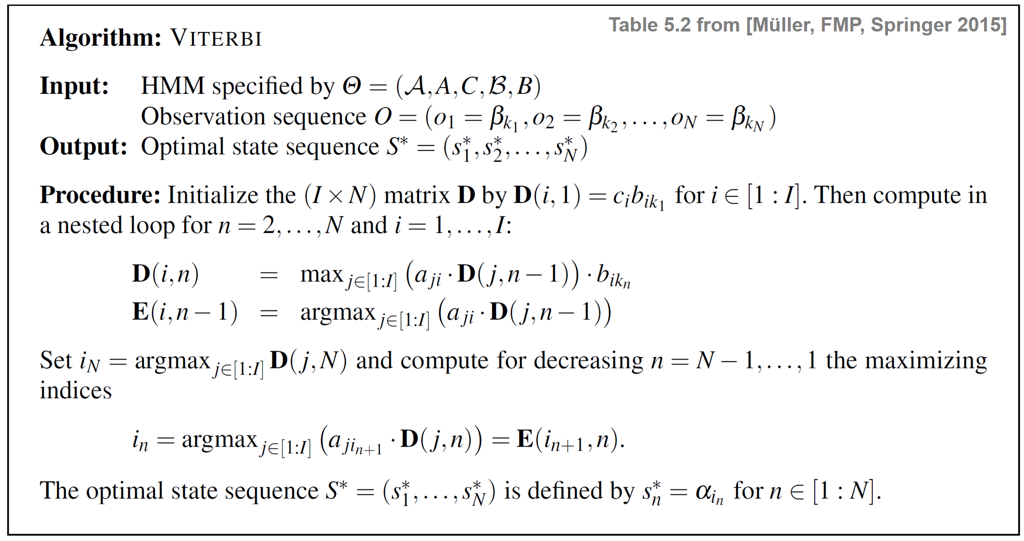
- 다음 그림은 Viterbi 알고리즘의 주요 단계를 보여준다.
- 파란색 셀은 알고리즘의 초기화 역할을 하는 \(\mathbf{D}(i,1)\) 항목을 나타낸다.
- 빨간색 셀은 주 반복(main iteration) 의 계산을 나타낸다.
- 검은색 셀은 최적의 상태 시퀀스를 얻기 위해 역 추적에 사용되는 최대화 인덱스를 나타낸다.
- 행렬 \(E\)는 재귀에서 최대화 인덱스를 추적하는 데 사용된다. 이 정보는 두 번째 단계에서 백트래킹(backtracking) 을 사용하여 최적의 상태 시퀀스를 구성할 때 필요하다.
ipd.Image("../img/6.chord_recognition/FMP_C5_F27.png", width=600)
전체 절차는 DTW 알고리즘과 유사하며, 먼저 누적 비용 매트릭스를 구성한 다음 백트래킹을 사용하여 최적의 워핑 경로를 얻는다.
앞의 그림과 같이 Viterbi 알고리즘은 각각 \(I\)개 노드(상태)로 구성된 \(N\)개 레이어로 그래프와 같은 구조를 구축하는 반복적인 방식으로 진행된다.
또한 두 개의 이웃 레이어는 \(I^2\) 에지로 연결되며, 이는 주어진 레이어에서 새 레이어를 구성하는 데 필요한 작업 수의 순서도 결정한다.
이로부터 Viterbi 알고리즘의 계산 복잡도는 \(O(N\cdot I^2)\)로, 나이브한 접근에 필요한 \(O(I^N)\)보다 훨씬 낫다.
예시
ipd.display(ipd.Image("../img/6.chord_recognition/FMP_C5_F28a.png", width=700))
ipd.display(ipd.Image("../img/6.chord_recognition/FMP_C5_F28b.png", width=700))

Viterbi 알고리즘 실행
def viterbi(A, C, B, O):
"""Viterbi algorithm for solving the uncovering problem
Args:
A (np.ndarray): State transition probability matrix of dimension I x I
C (np.ndarray): Initial state distribution of dimension I
B (np.ndarray): Output probability matrix of dimension I x K
O (np.ndarray): Observation sequence of length N
Returns:
S_opt (np.ndarray): Optimal state sequence of length N
D (np.ndarray): Accumulated probability matrix
E (np.ndarray): Backtracking matrix
"""
I = A.shape[0] # Number of states
N = len(O) # Length of observation sequence
# Initialize D and E matrices
D = np.zeros((I, N))
E = np.zeros((I, N-1)).astype(np.int32)
D[:, 0] = np.multiply(C, B[:, O[0]])
# Compute D and E in a nested loop
for n in range(1, N):
for i in range(I):
temp_product = np.multiply(A[:, i], D[:, n-1])
D[i, n] = np.max(temp_product) * B[i, O[n]]
E[i, n-1] = np.argmax(temp_product)
# Backtracking
S_opt = np.zeros(N).astype(np.int32)
S_opt[-1] = np.argmax(D[:, -1])
for n in range(N-2, -1, -1):
S_opt[n] = E[int(S_opt[n+1]), n]
return S_opt, D, E# Define model parameters
A = np.array([[0.8, 0.1, 0.1],
              [0.2, 0.7, 0.1],
              [0.1, 0.3, 0.6]])
C = np.array([0.6, 0.2, 0.2])
B = np.array([[0.7, 0.0, 0.3],
              [0.1, 0.9, 0.0],
              [0.0, 0.2, 0.8]])
O = np.array([0, 2, 0, 2, 2, 1]).astype(np.int32)
#O = np.array([1]).astype(np.int32)
#O = np.array([1, 2, 0, 2, 2, 1]).astype(np.int32)
# Apply Viterbi algorithm
S_opt, D, E = viterbi(A, C, B, O)
#
print('Observation sequence: O = ', O)
print('Optimal state sequence: S = ', S_opt)
np.set_printoptions(formatter={'float': "{: 7.4f}".format})
print('D =', D, sep='\n')
np.set_printoptions(formatter={'float': "{: 7.0f}".format})
print('E =', E, sep='\n')Observation sequence: O = [0 2 0 2 2 1]
Optimal state sequence: S = [0 0 0 2 2 1]
D =
[[ 0.4200 0.1008 0.0564 0.0135 0.0033 0.0000]
[ 0.0200 0.0000 0.0010 0.0000 0.0000 0.0006]
[ 0.0000 0.0336 0.0000 0.0045 0.0022 0.0003]]
E =
[[0 0 0 0 0]
[0 0 0 0 2]
[0 2 0 2 2]]Viterbi Algorithm의 log-domain 실행
- Viterbi 알고리즘의 각 반복에서 \(n-1\) 단계에서 누적된 \(\mathbf{D}\)의 확률값에 \(A\)와 \(B\)의 두 확률값을 곱한다.
- 더 정확하게는 다음과 같다.
\[\mathbf{D}(i,n) = \max_{j\in[1:I]}\big(a_{ij} \cdot\mathbf{D}(j,n-1) \big) \cdot b_ {i_{k_n}}\]
모든 확률 값은 \([0,1]\) 구간에 있기 때문에 이러한 값의 곱은 반복 횟수 \(n\)에 따라 기하급수적으로 감소한다. 결과적으로 \(N\)이 큰 입력 시퀀스 \(O=(o_{1},o_{2},\ldots o_{N})\)의 경우 \(\mathbf{D}\)의 값은 매우 작아지며, 결국 수치적 언더플로(underflow)로 이어질 수 있다.
확률 값의 곱을 다룰 때 잘 알려진 트릭은 log-domain에서 작업하는 것이다. 이를 위해 모든 확률 값에 로그를 적용하고 곱셈을 합산으로 대체한다. 로그는 강한 단조 함수이기 때문에 순서 관계는 로그 도메인에서 보존되어 최대화 또는 최소화와 같은 작업을 전달할 수 있다.
다음 코드 셀에서는 Viterbi 알고리즘의 로그 변형을 제공한다. 이 변형은 누적 로그 확률 행렬 \(\log(\mathbf{D})\) (
D_log)(로그가 각 항목에 적용됨)뿐만 아니라 원래 알고리즘과 정확히 동일한 최적 상태 시퀀스 \(S^\ast\) 및 동일한 백트래킹 행렬 \(E\)를 생성한다. 또한 온전성 검사로서 계산된 로그 행렬D_log에 지수 함수를 적용하여 위의 원래 Viterbi 알고리즘에 의해 계산된 행렬D를 산출해야 한다.
def viterbi_log(A, C, B, O):
    """Viterbi algorithm (log variant) for solving the uncovering problem

    Args:
        A (np.ndarray): State transition probability matrix of dimension I x I
        C (np.ndarray): Initial state distribution  of dimension I
        B (np.ndarray): Output probability matrix of dimension I x K
        O (np.ndarray): Observation sequence of length N

    Returns:
        S_opt (np.ndarray): Optimal state sequence of length N
        D_log (np.ndarray): Accumulated log probability matrix
        E (np.ndarray): Backtracking matrix
    """
    I = A.shape[0]    # Number of states
    N = len(O)  # Length of observation sequence
    tiny = np.finfo(0.).tiny
    A_log = np.log(A + tiny)
    C_log = np.log(C + tiny)
    B_log = np.log(B + tiny)

    # Initialize D and E matrices
    D_log = np.zeros((I, N))
    E = np.zeros((I, N-1)).astype(np.int32)
    D_log[:, 0] = C_log + B_log[:, O[0]]

    # Compute D and E in a nested loop
    for n in range(1, N):
        for i in range(I):
            temp_sum = A_log[:, i] + D_log[:, n-1]
            D_log[i, n] = np.max(temp_sum) + B_log[i, O[n]]
            E[i, n-1] = np.argmax(temp_sum)

    # Backtracking
    S_opt = np.zeros(N).astype(np.int32)
    S_opt[-1] = np.argmax(D_log[:, -1])
    for n in range(N-2, -1, -1):
        S_opt[n] = E[int(S_opt[n+1]), n]

    return S_opt, D_log, E
# Apply Viterbi algorithm (log variant)
S_opt, D_log, E = viterbi_log(A, C, B, O)
print('Observation sequence: O = ', O)
print('Optimal state sequence: S = ', S_opt)
np.set_printoptions(formatter={'float': "{: 7.2f}".format})
print('D_log =', D_log, sep='\n')
np.set_printoptions(formatter={'float': "{: 7.4f}".format})
print('exp(D_log) =', np.exp(D_log), sep='\n')
np.set_printoptions(formatter={'float': "{: 7.0f}".format})
print('E =', E, sep='\n')Observation sequence: O = [0 2 0 2 2 1]
Optimal state sequence: S = [0 0 0 2 2 1]
D_log =
[[ -0.87 -2.29 -2.87 -4.30 -5.73 -714.35]
[ -3.91 -711.57 -6.90 -713.57 -715.00 -7.44]
[-710.01 -3.39 -712.30 -5.40 -6.13 -8.25]]
exp(D_log) =
[[ 0.4200 0.1008 0.0564 0.0135 0.0033 0.0000]
[ 0.0200 0.0000 0.0010 0.0000 0.0000 0.0006]
[ 0.0000 0.0336 0.0000 0.0045 0.0022 0.0003]]
E =
[[0 0 0 0 0]
[0 0 0 0 2]
[0 2 0 2 2]]HMM 기반 화음 인식(Chord Recognition)
HMM이 어떻게 자동 화음 인식을 개선하는데 적용될 수 있는지 알아보자.
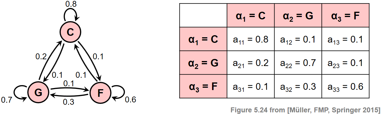
우선, 화음 인식 문제에 적합한 HMM 모델을 만들어야 한다. 보통 HMM은 매개변수 \(\Theta:=(\mathcal{A},A,C,\mathcal{B},B)\)에 의해 구체화 된다.
화음 인식의 맥락에서 다음의 상태 집합은 화음 인식에서 허용되는 여러 화음 유형을 모델링하는데 사용된다. \[\mathcal{A}:=\{\alpha_{1},\alpha_{2},\ldots,\alpha_{I}\}\]
템플릿-기반 화음 인식에서 그랬듯이, 여기서도 12 장3화음과 12 단3화음만 고려한다. \[\mathcal{A} = \{\mathbf{C},\mathbf{C}^\sharp,\ldots,\mathbf{B},\mathbf{Cm},\mathbf{Cm^\sharp},\ldots,\mathbf{Bm}\}\]
이 경우 HMM은 \(I=24\) 개 상태로 구성된다. 예를 들어 \(\alpha_{1}\)는 \(\mathbf{C}\)에 해당하고 \(\alpha_{13}\)는 \(\mathbf{Cm}\)에 해당한다.
또한 다음을 수행한다.
- 먼저, 음악적으로 정보를 얻는 방식으로 다른 HMM 매개변수를 지정하여 HMM을 명시적으로 생성하는 방법을 설명한다. 이러한 매개변수는 Baum-Welch 알고리즘을 사용하여 훈련 데이터에서 자동으로 학습될 수 있지만, HMM 매개변수의 수동적인 지정은 교육적이며 명시적인 음악적 의미를 가진 HMM으로 이끌 수 있다.
- 둘째, 이 HMM을 화음 인식에 적용한다. HMM의 입력(즉, 관찰 시퀀스)은 음악 녹음의 크로마그램 표현이다. Viterbi 알고리즘을 적용하여 크로마 시퀀스를 가장 잘 설명하는 최적의 상태 시퀀스(화음 레이블로 구성됨)를 도출한다. 화음 라벨의 시퀀스는 프레임별 화음 인식 결과를 산출한다.
HMM 기반의 화음 인식 결과와 템플릿 기반 접근 방식의 결과를 비교한다. 특히 HMM 전환 모델이 일종의 context-aware postfiltering(맥락을 인식하는 사후필터링)의 역할을 하는 것을 볼 수 있다.
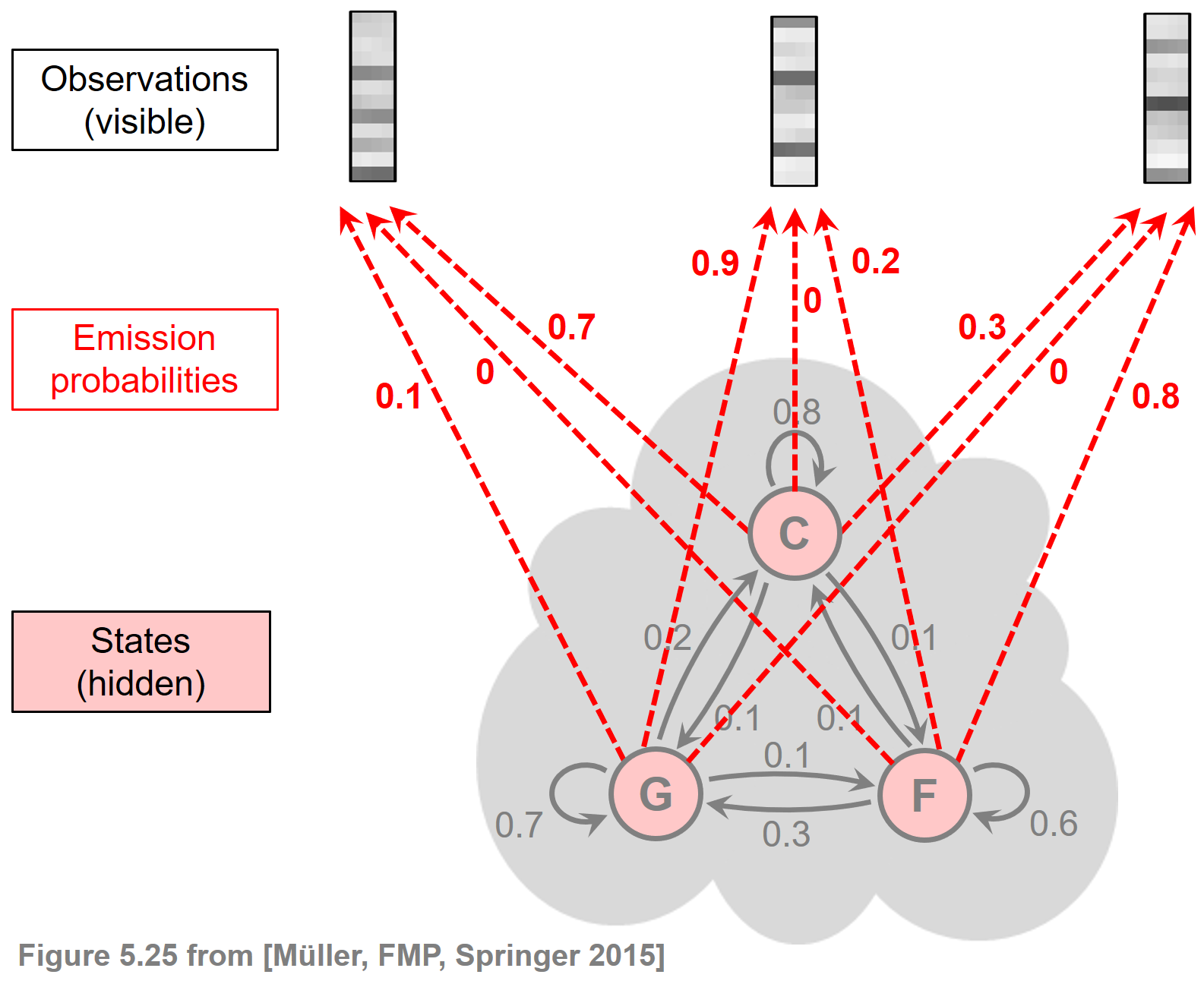
방출 우도의 구체화 (Specification of Emission Likelihoods)
화음 인식 시나리오에서 관측값(observations)은 주어진 오디오 녹음에서 이전에 추출된 크로마 벡터이다. 즉, 관측값은 연속적인 특징 공간 \(\mathcal{F}=\mathbb{R}^{12}\)의 요소인 \(12\)차원의 실수 벡터이다.
지금까지는 관측값이 유한 출력 공간 \(\mathcal{B}\)에서 나오는 이산 기호인 이산(discrete) HMM의 경우만 고려했다. 이산 HMM을 시나리오에 적용하기 위해 가능한 절차 중 하나는 소위 코드북(codebook) 이라고 하는 프로토타입 벡터의 유한 세트를 도입하는 것이다. 이러한 코드북은 연속적인 특징 공간 \(\mathcal{F}=\mathbb{R}^{12}\)의 이산화로 간주될 수 있으며, 여기서 각 코드북 벡터는 전체 범위의 특징 벡터를 나타낸다. 그런 다음 이 유한한 코드북 벡터 세트를 기반으로 방출 확률(emission probability)을 결정할 수 있다.
대안으로 다음 HMM 변형에서 이산 출력 공간 \(\mathcal{B}\)를 연속적인 특징 공간 \(\mathcal{F}=\mathbb{R}^{12}\) 및 우도 함수(likelihood functions) 에 의한 방출 확률 행렬 \(B\)로 대체한다. 특히, 주어진 상태의 방출 확률은 state-dependent한 정규화된 템플릿과 정규화된 관측(크로마) 벡터의 내적으로 정의되는 정규화된 유사성(similarity) 값으로 대체된다.
\(s:\mathcal{F} \times \mathcal{F} \to [0,1]\)를 정규화된 크로미 벡터의 내적에 의해 정의된 유사도 측정(similarity measure) 이라고 하자(단, 0으로 나누지 못하도록 임계값을 설정한 정규화 사용): \[s(x, y) = \frac{\langle x,y\rangle}{\|x\|_2\cdot\|y\|_2}\] for \(x,y\in\mathcal{F}\)
\(I=24\)개의 장,단3화음 (상태 \(\mathcal{A}\)로 인코딩되고 \([1:I]\) 집합으로 인덱싱됨)을 기반으로 이진 화음 템플릿(binary chord templates) \(\mathbf{t}_i\in \mathcal{F}\) for \(i\in [1:I]\)을 고려한다.
그런 다음 state-dependent likelihood function \(b_i:\mathcal{F}\to [0,1]\)를 다음과 같이 정의한다. \[b_i(x) := \frac{s(x, \mathbf{t}_i)}{\sum_{j\in[1:I]}s(x, \mathbf{t}_j)}\] for \(x\in\mathcal{F}\) and \(i\in [1:I]\)
시나리오에서 관측 시퀀스 \(O=(o_{1},o_{2},\ldots,o_{N})\)는 크로마 벡터 \(o_n\in\mathcal{F}\)의 시퀀스이다.
관측-종속적인 \((I\times N)\)-행렬 \(B[O]\)를 다음과 같이 정의한다. \[B[O](i,n) = b_i(o_n)\] for \(i\in[1:I]\) and \(n\in[1:N]\)
행렬은 템플릿 기반 화음 인식에 대한 설명에서 소개되었듯이, 시간-화음 표현의 형태로 시각화된 column-wise \(\ell^1\)-정규화를 사용하는 화음 유사성 행렬(chord similarity matrix) 이다. Viterbi 알고리즘의 맥락에서 likelihood \(B[O](i,n)\)는 확률 값 \(b_{ik_n}\)를 대체하는 데 사용된다.
ipd.display(ipd.Image("../img/6.chord_recognition/FMP_C5_F20a.png", width=500))
ipd.display(ipd.Audio("../data_FMP/FMP_C5_F20_Bach_BWV846-mm1-4_Fischer.wav"))
# Specify
fn_wav = "../data_FMP/FMP_C5_F20_Bach_BWV846-mm1-4_Fischer.wav"
fn_ann = "../data_FMP/FMP_C5_F20_Bach_BWV846-mm1-4_Fischer_ChordAnnotations.csv"
color_ann = {'C': [1, 0.5, 0, 1], 'G': [0, 1, 0, 1], 'Dm': [1, 0, 0, 1], 'N': [1, 1, 1, 1]}

N = 4096
H = 1024
X, Fs_X, x, Fs, x_dur = \
    compute_chromagram_from_filename(fn_wav, N=N, H=H, gamma=0.1, version='STFT')
N_X = X.shape[1]

# Chord recogntion
chord_sim, chord_max = chord_recognition_template(X, norm_sim='1')
chord_labels = get_chord_labels(nonchord=False)

# Annotations
chord_labels = get_chord_labels(ext_minor='m', nonchord=False)
ann_matrix, ann_frame, ann_seg_frame, ann_seg_ind, ann_seg_sec = convert_chord_ann_matrix(
    fn_ann, chord_labels, Fs=Fs_X, N=N_X, last=True)
#P, R, F, TP, FP, FN = compute_eval_measures(ann_matrix, chord_max)
# Plot
cmap = compressed_gray_cmap(alpha=1, reverse=False)
fig, ax = plt.subplots(3, 2, gridspec_kw={'width_ratios': [1, 0.03],
'height_ratios': [1.5, 3, 0.2]}, figsize=(8, 6))
plot_chromagram(X, ax=[ax[0, 0], ax[0, 1]], Fs=Fs_X, clim=[0, 1], xlabel='',
title='Observation sequence (chromagram with feature rate = %0.1f Hz)' % (Fs_X))
plot_segments_overlay(ann_seg_sec, ax=ax[0, 0], time_max=x_dur,
print_labels=False, colors=color_ann, alpha=0.1)
plot_matrix(chord_sim, ax=[ax[1, 0], ax[1, 1]], Fs=Fs_X, clim=[0, np.max(chord_sim)],
title='Likelihood matrix (time–chord representation)',
ylabel='Chord', xlabel='')
ax[1, 0].set_yticks(np.arange(len(chord_labels)))
ax[1, 0].set_yticklabels(chord_labels)
plot_segments_overlay(ann_seg_sec, ax=ax[1, 0], time_max=x_dur,
print_labels=False, colors=color_ann, alpha=0.1)
plot_segments(ann_seg_sec, ax=ax[2, 0], time_max=x_dur, time_label='Time (seconds)',
colors=color_ann, alpha=0.3)
ax[2,1].axis('off')
plt.tight_layout()
전이 확률의 구체화 (Specification of Transition Probabilities)
음악에서 특정 화음 전환은 다른 화음 전환보다 더 자주 발생하기 마련이다. 따라서 HMM을 사용할 수 있으며, 다양한 화음 사이의 1차(first-oreder) 시간(temporal) 관계는 전이 확률 행렬(transition probability matrix) \(A\)로 캡처할 수 있다.
다음에서 \(\alpha_{i}\rightarrow\alpha_{j}\) 표기법을 사용하여 \(\alpha_{i}\) 상태에서 \(\alpha_{j}\) 상태로 전환하는 것을 나타낸다. (for \(i,j\in[1:I]\))
예를 들어, 계수 \(a_{1,2}\)는 전환 \(\alpha_{1}\rightarrow\alpha_{2}\)(\(\mathbf{C}\rightarrow\mathbf{C} ^\sharp\)에 해당)의 확률을 표현하고, 반면 \(a_{1,8}\)는 \(\alpha_{1}\rightarrow\alpha_{8}\)(\(\mathbf{C}\rightarrow\mathbf{G}\)에 해당)의 확률을 나타낸다.
실제 음악에서는 으뜸음(tonic)에서 딸림음(dominant)으로의 변화가 반음 하나 변화하는 것보다 훨씬 더 많으므로 \(a_{1,8}\)는 \(a_{1,2}\)보다 훨씬 커야 한다.
계수 \(a_{i,i}\)는 \(\alpha_{i}\)(for \(i\in[1:I]\)) (즉, \(\alpha_{i}\rightarrow\alpha_{i}\)) 상태에 머무를 확률을 나타낸다. 이러한 계수는 자기 전이(self-transition) 확률이라고도 한다.
전이 확률 행렬은 여러 가지 방법으로 구체화될 수 있다.
- 예를 들어, 행렬은 화성 이론(harmony theory)의 규칙에 따라 음악 전문가가 수동으로 정의할 수 있다. 가장 일반적인 접근 방식은 레이블이 지정된 데이터에서 전환 확률을 추정하여 이러한 행렬을 자동으로 생성하는 것이다.
다음 그림에서는 세 가지 다른 전이 행렬을 보여준다(시각화 목적으로 로그 확률 척도를 사용).
- 첫 번째는 비틀즈 컬렉션을 기반으로 레이블이 지정된 프레임 시퀀스에서 바이그램(bigram)(인접 요소 쌍)을 사용하여 레이블이 지정된 훈련 데이터에서 학습되었다. 예를 들어 계수 \(a_{1,8}\)(전환 \(\mathbf{C}\rightarrow\mathbf{G}\)에 해당)가 강조 표시되어있다.
- 두 번째 행렬은 이전 행렬에서 얻은 조옮김 불변(transposition-invariant) 전이 확률 행렬이다. 조옮김 불변성을 달성하기 위해 레이블이 지정된 훈련 데이터 세트는 고려되는 바이그램에 대해 가능한 모든 12개의 순환 크로마 이동(cyclic chroma shifts)을 고려하여 보강된다.
- 세 번째 행렬은 주 대각선(자기 전이)에서 큰 값을 갖고 나머지 모든 위치에서 훨씬 작은 값을 갖는 균일(uniform) 전이 확률 행렬이다.
ipd.Image("../img/6.chord_recognition/FMP_C5_F29-30-32.png")
- 다음 코드 셀에서 비틀즈 컬렉션을 기반으로 추정된(6.4.에서 이를 다루기로 함) 미리 계산된 전환 행렬이 포함된
CSV파일을 읽는다. 그림에서는 확률 값과 로그 확률 값을 모두 표시한다.
def plot_transition_matrix(A, log=True, ax=None, figsize=(6, 5), title='',
                           xlabel='State (chord label)', ylabel='State (chord label)',
                           cmap='gray_r', quadrant=False):
    """Plot a transition matrix for 24 chord models (12 major and 12 minor triads)

    Args:
        A: Transition matrix
        log: Show log probabilities (Default value = True)
        ax: Axis (Default value = None)
        figsize: Width, height in inches (only used when ax=None) (Default value = (6, 5))
        title: Title for plot (Default value = '')
        xlabel: Label for x-axis (Default value = 'State (chord label)')
        ylabel: Label for y-axis (Default value = 'State (chord label)')
        cmap: Color map (Default value = 'gray_r')
        quadrant: Plots additional lines for C-major and C-minor quadrants (Default value = False)

    Returns:
        fig: The created matplotlib figure or None if ax was given.
        ax: The used axes.
        im: The image plot
    """
    fig = None
    if ax is None:
        fig, ax = plt.subplots(1, 1, figsize=figsize)
        ax = [ax]

    if log is True:
        A_plot = np.log(A)
        cbar_label = 'Log probability'
        clim = [-6, 0]
    else:
        A_plot = A
        cbar_label = 'Probability'
        clim = [0, 1]
    im = ax[0].imshow(A_plot, origin='lower', aspect='equal', cmap=cmap, interpolation='nearest')
    im.set_clim(clim)
    plt.sca(ax[0])
    cbar = plt.colorbar(im)
    ax[0].set_xlabel(xlabel)
    ax[0].set_ylabel(ylabel)
    ax[0].set_title(title)
    cbar.ax.set_ylabel(cbar_label)

    chord_labels = get_chord_labels()
    chord_labels_squeezed = chord_labels.copy()
    for k in [1, 3, 6, 8, 10, 11, 13, 15, 17, 18, 20, 22]:
        chord_labels_squeezed[k] = ''

    ax[0].set_xticks(np.arange(24))
    ax[0].set_yticks(np.arange(24))
    ax[0].set_xticklabels(chord_labels_squeezed)
    ax[0].set_yticklabels(chord_labels)

    if quadrant is True:
        ax[0].axvline(x=11.5, ymin=0, ymax=24, linewidth=2, color='r')
        ax[0].axhline(y=11.5, xmin=0, xmax=24, linewidth=2, color='r')

    return fig, ax, im
# Load transition matrix estimated on the basis of the Beatles collection
fn_csv = '../data_FMP/FMP_C5_transitionMatrix_Beatles.csv'
A_est_df = pd.read_csv(fn_csv, delimiter=';')
A_est = A_est_df.to_numpy('float64')
fig, ax = plt.subplots(1, 2, gridspec_kw={'width_ratios': [1, 1],
'height_ratios': [1]},
figsize=(10, 3.8))
plot_transition_matrix(A_est, log=False, ax=[ax[0]], title='Transition matrix')
plot_transition_matrix(A_est, ax=[ax[1]], title='Transition matrix with log probabilities')
plt.tight_layout()
- 조옮김-불변 전이 행렬 (transposition-invariant transition matrix)을 얻기 위해 원래 행렬의 4개 사분면(장화음, 단화음 영역으로 정의됨)을 순환 이동하고 평균화하여 행렬 수준에서 순환 크로마 이동을 시뮬레이션한다.
- 그림에서 원본의 전이 행렬과 결과의 옮김-불변 전이 행렬을 보여준다.
def matrix_circular_mean(A):
    """Computes circulant matrix with mean diagonal sums

    Args:
        A (np.ndarray): Square matrix

    Returns:
        A_mean (np.ndarray): Circulant output matrix
    """
    N = A.shape[0]
    A_shear = np.zeros((N, N))
    for n in range(N):
        A_shear[:, n] = np.roll(A[:, n], -n)
    circ_sum = np.sum(A_shear, axis=1)
    A_mean = circulant(circ_sum) / N
    return A_mean


def matrix_chord24_trans_inv(A):
    """Computes transposition-invariant matrix for transition matrix
    based 12 major chords and 12 minor chords

    Args:
        A (np.ndarray): Input transition matrix

    Returns:
        A_ti (np.ndarray): Output transition matrix
    """
    A_ti = np.zeros(A.shape)
    A_ti[0:12, 0:12] = matrix_circular_mean(A[0:12, 0:12])
    A_ti[0:12, 12:24] = matrix_circular_mean(A[0:12, 12:24])
    A_ti[12:24, 0:12] = matrix_circular_mean(A[12:24, 0:12])
    A_ti[12:24, 12:24] = matrix_circular_mean(A[12:24, 12:24])
    return A_ti
A_ti = matrix_chord24_trans_inv(A_est)
fig, ax = plt.subplots(1, 2, gridspec_kw={'width_ratios': [1, 1],
'height_ratios': [1]},
figsize=(10, 3.8))
plot_transition_matrix(A_est, ax=[ax[0]], quadrant=True,
title='Transition matrix')
plot_transition_matrix(A_ti, ax=[ax[1]], quadrant=True,
title='Transposition-invariant transition matrix')
plt.tight_layout()
- 마지막으로 uniform 전이 확률 행렬을 생성하는 기능을 보자. 이 함수에는 자기 전이 확률(주대각선의 값)을 결정하는 매개변수 \(p\in[0,1]\)가 있다. 나머지 위치에 대한 확률은 결과 행렬이 확률 행렬(즉, 모든 행과 열의 합이 1이 됨)이 되도록 설정한다.
def uniform_transition_matrix(p=0.01, N=24):
    """Computes uniform transition matrix

    Args:
        p (float): Self transition probability (Default value = 0.01)
        N (int): Column and row dimension (Default value = 24)

    Returns:
        A (np.ndarray): Output transition matrix
    """
    off_diag_entries = (1-p) / (N-1)     # rows should sum up to 1
    A = off_diag_entries * np.ones([N, N])
    np.fill_diagonal(A, p)
    return A
fig, ax = plt.subplots(1, 2, gridspec_kw={'width_ratios': [1, 1],
'height_ratios': [1]},
figsize=(10, 3.8))
p = 0.5
A_uni = uniform_transition_matrix(p)
plot_transition_matrix(A_uni, ax=[ax[0]], title='Uniform transition matrix (p=%0.2f)' % p)
p = 0.9
A_uni = uniform_transition_matrix(p)
plot_transition_matrix(A_uni, ax=[ax[1]], title='Uniform transition matrix (p=%0.2f)' % p)
plt.tight_layout()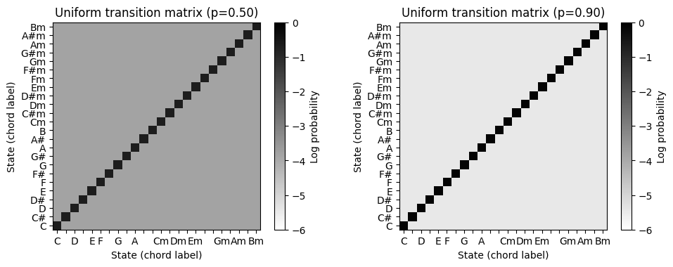
HMM 기반 화음 인식 (HMM-Based Chord Recognition)
앞에서 설명한 것처럼 HMM 기반 모델의 자유 매개변수는 훈련 세트에서 자동으로 학습하거나 음악적 지식을 사용하여 수동으로 설정할 수 있다.
Bach 예제를 계속 사용하여 HMM을 화음 인식 시나리오에 적용한 효과를 본다. 다음 설정을 사용한다.
- 관찰 시퀀스 \(O\)으로, 크로마 벡터 시퀀스를 사용한다.
- 전이 확률 행렬 \(A\)는 균일(uniform) 전이 행렬을 사용한다.
- 초기 상태 확률 벡터 \(C\)는 균일 분포를 사용한다.
- 방출(emission) 확률 행렬 \(B\)는 템플릿 기반 화음 인식에도 사용되는 화음 유사성 행렬의 정규화된 버전인 liklihood 행렬 \(B[O]\)로 대체한다.
- 프레임별 화음 인식 결과는 Viterbi 알고리즘에 의해 계산된 상태 시퀀스에 의해 제공된다.
방출 확률 대신 likelihood 행렬 \(B[O]\)를 사용하려면 원래 알고리즘을 약간 수정해야 한다. 다음 코드 셀에서는 수치적으로 안정적인 로그 버전을 사용하여 수정한다. 그런 다음 HMM 기반 결과와 템플릿 기반 접근 방식을 비교하여 평가 결과를 시간-화음 시각화 형태로 각각 보여준다.
def viterbi_log_likelihood(A, C, B_O):
    """Viterbi algorithm (log variant) for solving the uncovering problem

    Args:
        A (np.ndarray): State transition probability matrix of dimension I x I
        C (np.ndarray): Initial state distribution  of dimension I
        B_O (np.ndarray): Likelihood matrix of dimension I x N

    Returns:
        S_opt (np.ndarray): Optimal state sequence of length N
        S_mat (np.ndarray): Binary matrix representation of optimal state sequence
        D_log (np.ndarray): Accumulated log probability matrix
        E (np.ndarray): Backtracking matrix
    """
    I = A.shape[0]    # Number of states
    N = B_O.shape[1]  # Length of observation sequence
    tiny = np.finfo(0.).tiny
    A_log = np.log(A + tiny)
    C_log = np.log(C + tiny)
    B_O_log = np.log(B_O + tiny)

    # Initialize D and E matrices
    D_log = np.zeros((I, N))
    E = np.zeros((I, N-1)).astype(np.int32)
    D_log[:, 0] = C_log + B_O_log[:, 0]

    # Compute D and E in a nested loop
    for n in range(1, N):
        for i in range(I):
            temp_sum = A_log[:, i] + D_log[:, n-1]
            D_log[i, n] = np.max(temp_sum) + B_O_log[i, n]
            E[i, n-1] = np.argmax(temp_sum)

    # Backtracking
    S_opt = np.zeros(N).astype(np.int32)
    S_opt[-1] = np.argmax(D_log[:, -1])
    for n in range(N-2, -1, -1):
        S_opt[n] = E[int(S_opt[n+1]), n]

    # Matrix representation of result
    S_mat = np.zeros((I, N)).astype(np.int32)
    for n in range(N):
        S_mat[S_opt[n], n] = 1

    return S_mat, S_opt, D_log, E
A = uniform_transition_matrix(p=0.5)
C = 1 / 24 * np.ones((1, 24))
B_O = chord_sim
chord_HMM, _, _, _ = viterbi_log_likelihood(A, C, B_O)
P, R, F, TP, FP, FN = compute_eval_measures(ann_matrix, chord_HMM)
title = 'HMM-Based approach (N=%d, TP=%d, FP=%d, FN=%d, P=%.2f, R=%.2f, F=%.2f)' % (N_X, TP, FP, FN, P, R, F)
fig, ax, im = plot_matrix_chord_eval(ann_matrix, chord_HMM, Fs=1,
title=title, ylabel='Chord', xlabel='Time (frames)', chord_labels=chord_labels)
plt.tight_layout()
plt.show()
P, R, F, TP, FP, FN = compute_eval_measures(ann_matrix, chord_max)
title = 'Template-based approach (N=%d, TP=%d, FP=%d, FN=%d, P=%.2f, R=%.2f, F=%.2f)' %\
(N_X, TP, FP, FN, P, R, F)
fig, ax, im = plot_matrix_chord_eval(ann_matrix, chord_max, Fs=1,
title=title, ylabel='Chord', xlabel='Time (frames)', chord_labels=chord_labels)
plt.tight_layout()
plt.show()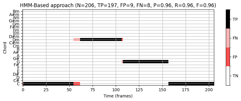
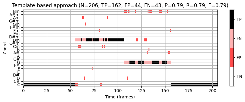
이 예에서는 HMM 기반 화음 인식기가 템플릿 기반 접근 방식보다 우수하다.
HMM 기반 접근 방식의 개선은 특히 상황에 맞는 평활화(smoothing)를 도입하는 전이 모델(transition model) 에서 비롯된다. 높은 자기-전이 확률의 경우, 화음 인식기는 다른 화음으로 변경하기보다 현재 화음에 머무르는 경향이 있으며, 이는 일종의 평활화라고 볼 수 있다. 이 효과는 깨진(broken) 화음이 짧은 시간의 많은 화음 모호성을 유발하는 Bach 예제에서도 입증된다. 이러한 효과는 간단한 템플릿 기반 화음 인식기를 사용할 때 많은 무작위와 같은 화음 변경으로 이어지게 한다.
HMM 기반 접근 방식을 사용하면 상대적으로 낮은 전이 확률이 방출 확률의 충분한 증가로 보상되는 경우에만 화음 변경이 수행된다. 결과적으로 지배적인 화음 변경만 남는다.
사전 필터링 vs. 사후 필터링 (Prefiltering vs. Postfiltering)
화음 인식 평가에서 다룬 입력 크로마그램을 계산할 때 더 긴 윈도우 크기를 적용하여 개선을 달성할 수 있음을 Bach 예제로 보여주었다.
더 긴 윈도우 크기를 적용하면 관측 시퀀스의 시간적 평활화 정도가 더 많거나 적다. 이 평활화는 패턴 매칭 단계 이전에 수행되므로, 이 전략을 사전 필터링(prefiltering) 이라고도 한다. 이러한 사전 필터링 단계는 노이즈와 같은 프레임을 부드럽게 처리할 뿐만 아니라 특징적인 크로마 정보를 제거하고 전환을 흐리게 한다.
사전 필터링과 달리 HMM 기반 접근 방식은 특징(feature) 표현을 그대로 둔다. 또한, 평활화는 패턴 매칭 단계와 조합하여 수행된다. 이러한 이유로 이 접근 방식을 사후 필터링(postfiltering) 이라고도 한다. 결과적으로 원래 크로마 정보가 보존되고 특징 표현의 전환이 선명하게 유지된다.
ipd.Image("../img/6.chord_recognition/FMP_C5_F13.png", width=700)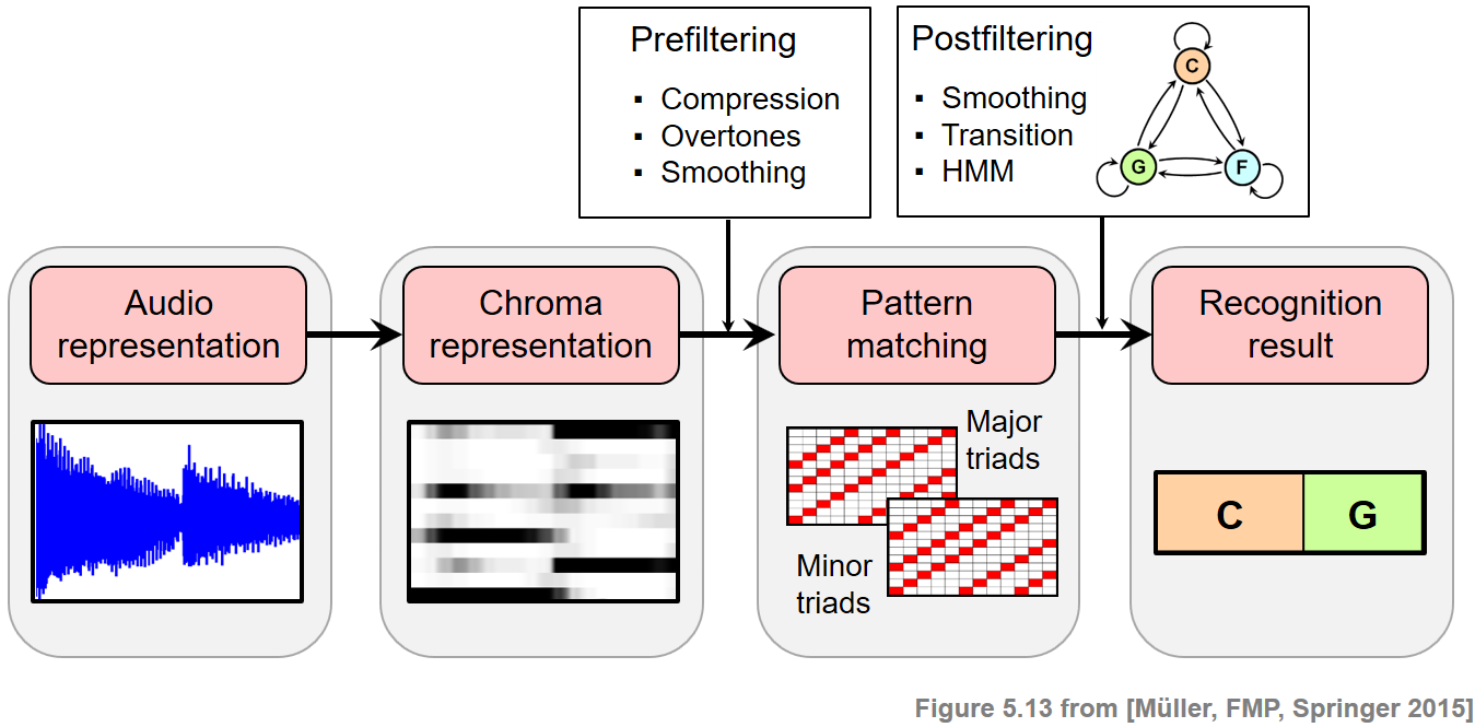
여기서는 기본적인 HMM 변형만 다루었지만, 여러가지 변형과 확장적인 HMM(e.g. 연속 HMMs, HMMs with specific state transition topologies)을 쓸 수도 있다. HMM은 모형 매개변수를 고정하는 대신 자동적으로 자유 매개변수를 학습시키는(e.g. Baum-Welch 알고리즘) 장점이 있다. 모델 매개변수를 수동으로 고정하는 대신 일반 HMM은 학습 예제를 기반으로 자유 매개변수를 자동으로 학습하는 것이다(예: [Baum-Welch 알고리즘] 사용).
참고: Hidden Markov Models for Speech Recognition by Huang et al. (1990).
ipd.Image("../img/6.chord_recognition/FMP_C5_F33.png" , width=600)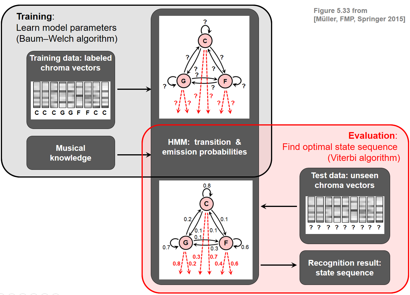
출처:
- https://www.audiolabs-erlangen.de/resources/MIR/FMP/C5/C5S3_HiddenMarkovModel.html
- https://www.audiolabs-erlangen.de/resources/MIR/FMP/C5/C5S3_Viterbi.html
- https://www.audiolabs-erlangen.de/resources/MIR/FMP/C5/C5S3_ChordRec_HMM.html
\(\leftarrow\) 6.2. 템플릿 기반 화음 인식